Per-patch loss-coupling, in plain words

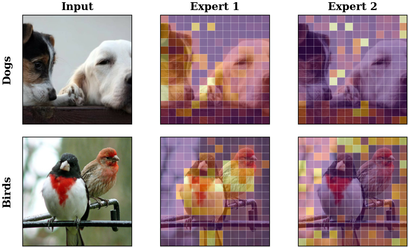
Start with the picture#

ExPLoRe is a method we published at ECCV 2026, with Maofeng Tang and my advisor Hairong Qi. It addresses a specific problem in masked image modeling. When a model pretrains with several losses at once, existing methods weight those losses with one global number each, and ExPLoRe replaces the global numbers with a separate learned weight for every image patch, reused from the routing weights that a Soft-MoE already computes. The full details live in the paper and the code, and this post walks through the idea, the ablations behind it, and the open questions in plainer language.

The image above shows per-patch dispatch weights from a 2-expert model trained from scratch on ImageNet, with learning signals that come only from a frozen CLIP teacher. After 300 epochs, one expert has learned to weight the loss heavily on the animal in each image while the other favors the background and context. The training setup contains no notion of foreground or background anywhere, so the split emerges entirely from loss gradients flowing into the router.

Why global scalars fall short#

The predecessor to this work, MEDiC, combined three masked-image-modeling signals in one student encoder, with CLIP token distillation, global CLS alignment, and pixel reconstruction trained jointly. The framework worked and the numbers were competitive, but the three losses were balanced by a single hand-tuned scalar each, shared across every image, patch, and epoch.

The trouble with that setup is that an image is not uniform. A patch full of texture, like grass or fur, produces a very different reconstruction error than a patch on a face, and a patch with strong semantic content, the eye of a bird for example, carries a very different distillation signal than a patch of sky. Weighting each loss with one global scalar assumes the optimal blend is the same everywhere on the image, and removing that assumption became the goal of the project.

Most of a year went into making the global scalars work harder, through attention-based masking that biases which patches the model must reconstruct, per-objective scheduling that phases the losses in at different epochs, and GradNorm for automatic gradient balancing. Roughly fifty hand-tuned configurations and many months of refreshing a Weights & Biases tab later, the k-NN line had barely moved. (That stretch shows up in a separate post on the PhD.)

The GradNorm result settled the question. GradNorm is the standard principled answer to weighting competing objectives in multi-task learning, normalizing gradient magnitudes across tasks and adapting at every step. On our Token+CLS setup it landed at 72.8% k-NN, below the static-weight baseline of 74.2%, and on Token+Pixel it collapsed entirely to 32.5%. That number stayed in the paper because a principled global method, run with an extensive hyperparameter search, falling below its own static baseline says something about the problem itself. The takeaway was that scalars are the wrong shape for spatially heterogeneous objectives, no matter how carefully they get tuned.

Soft-MoE dispatch weights, and the trick#

The pivot came from Soft-MoE (Puigcerver et al., 2023), which replaces some MLP layers in a transformer with a small set of expert networks and routes each patch to each expert through a soft, fully differentiable matrix. There are actually two such matrices, produced by softmax-normalizing the shared routing logits along two different axes.

• The dispatch matrix D is normalized over patches for each expert, so every expert’s weights across patches sum to one and describe how much each patch contributes to that expert’s input.
• The combine matrix C is normalized over experts for each patch, so every patch’s weights across experts sum to one and describe how much each expert contributes to that patch’s output.

The full architecture sits inside the student encoder at alternating ViT blocks 11, six MoE blocks and six vanilla blocks. The frozen CLIP teacher provides per-patch target features, the student’s MoE blocks process the visible patches, and the dispatch weights at the last MoE block get reused as per-patch loss coefficients.

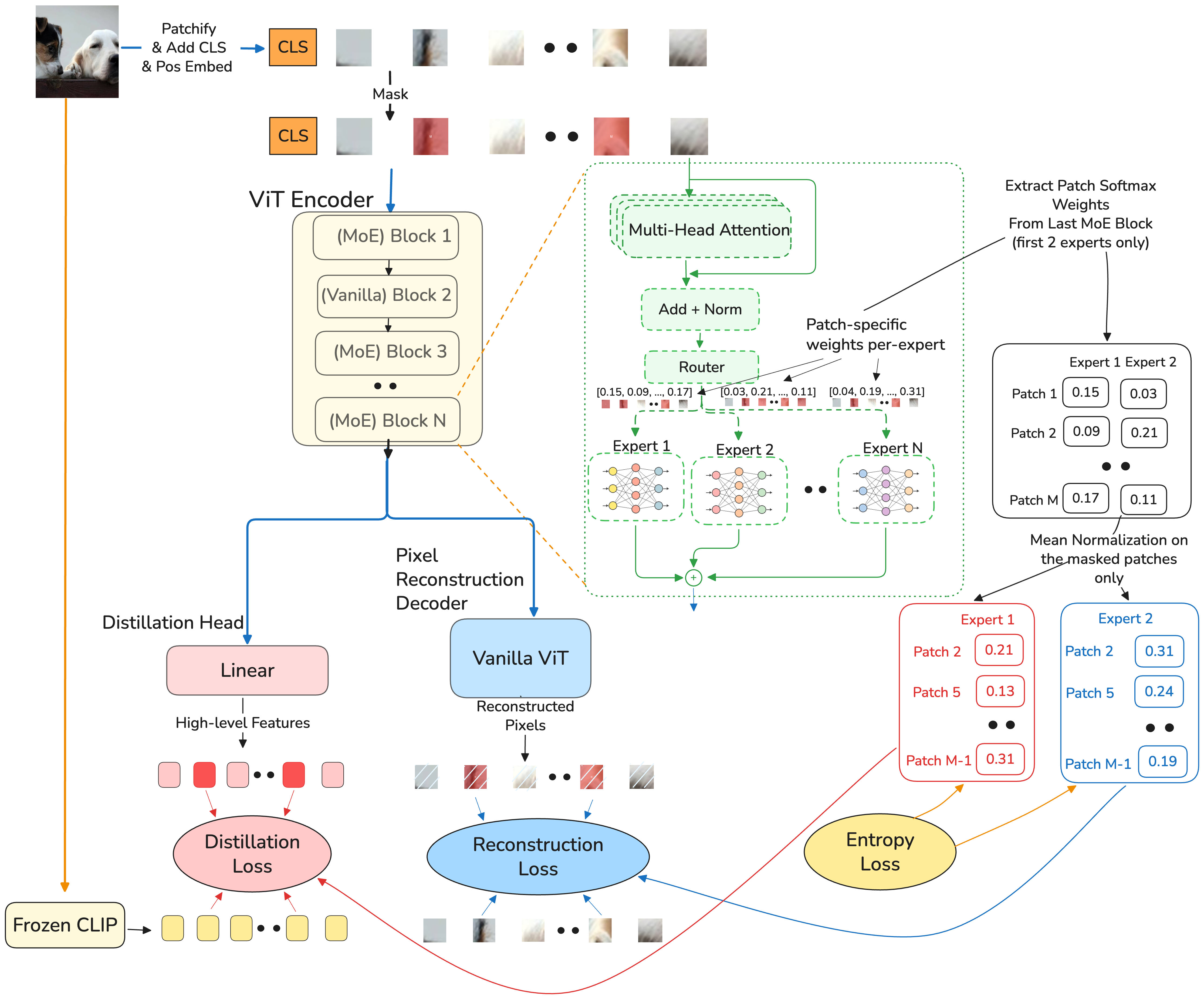
The trick is to let the dispatch weights double as per-patch loss weights. For E experts and K loss objectives, one expert is reserved per objective, and that objective’s per-patch loss gets scaled by the corresponding dispatch weight, so the router ends up setting the weight each loss gets on each patch.

The reason this works is what the paper calls loss-coupling. Because the dispatch weights are differentiable, the loss gradients flow back through the dispatch matrix to the router parameters themselves. On top of the usual MoE objective of routing tokens for capacity, the router also learns from how much its routing decisions affect each loss, and the equilibrium between those two pressures is content-dependent specialization.

Why the dispatch matrix does the weighting#

This small design choice turned out to carry the whole method. The obvious-looking variant came first, using the combine weights as the loss coefficients, since they are normalized per patch and resemble a natural probability distribution over experts for each patch’s loss. They hide a fatal degeneracy. Because their normalization runs over experts, the router can shrink the loss by pushing all combine weights toward zero on the patches that are hard to learn, so the loss shrinks while the model learns nothing. Combine-weight loss weighting falls to 2.1% k-NN, more than 70 points below the baseline, with the router zeroing the loss weights on the hard patches so the weighted loss vanishes while the underlying errors remain.

Dispatch weights close that loophole because their normalization runs over patches. Every expert’s dispatch weights sum to one across the image, so the router can shift weight between patches but has no way to zero everything out, and the per-patch comparison stays in absolute terms. Recognizing the degeneracy took a few months, and the fix ultimately came from staring at the two softmax axes long enough to notice how differently their failure modes behave.

The detach ablation#

Once the mechanism worked, the next question was whether the gains came from the mechanism or from the extra parameters. A 2-expert MoE has 116M parameters against 86M for the no-MoE baseline, and 30M of extra capacity could plausibly explain a lot on its own.

The clean test cuts just the gradient path. The loss is still computed with the dispatch weights as multipliers, but the weights are detached from the computation graph so that loss gradients can no longer reach the router, leaving the architecture, parameter count, compute, and MoE forward pass identical. With the coupling severed, k-NN drops from 75.4% to 73.8%, below even the 75.7% no-MoE baseline, so the extra capacity gives nothing back once the gradient path is gone. The unweighted MoE makes the same point from another angle. With dispatch weights computed but never used as loss coefficients, the model lands at 74.1% k-NN, again below the no-MoE baseline, so at this scale the extra experts actively hurt unless the coupling is there to organize them.

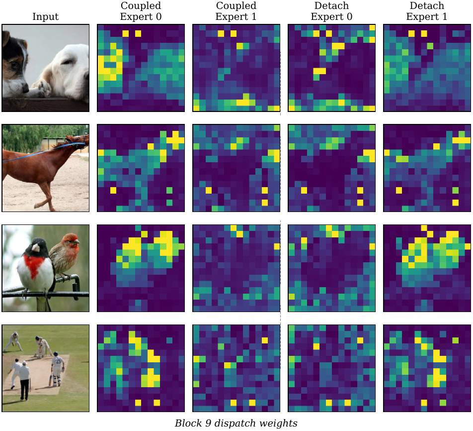
The figure above shows the same finding visually. Each row is a different image, the left two columns come from the loss-coupled model, and the right two come from the detach variant with the same backbone and training schedule. The coupled model produces spatially coherent, content-dependent routing, while the detach variant’s dispatch weights drift much closer to noise. The router still routes, since the forward MoE gradient still trains it, but it never learns that some patches matter more to the loss than others.

An emergent CLS specialist#

The paper’s routing analysis contains the finding that best illustrates what loss-coupling does. At block 11, the block whose dispatch weights feed the loss, Expert 1 concentrates 91 to 95% of its total dispatch weight on the CLS token alone. The CLS token is one of 197 tokens, so uniform routing would give it roughly half a percent.

None of this appears anywhere in the training setup. The model trains against a per-patch token-distillation loss and a global CLS-alignment loss, and the router is free to specialize however the gradients push it. The equilibrium it reaches makes one expert a de facto CLS specialist while the other covers the per-patch distillation across the rest of the image, matching the structure of the two losses. The concentration also appears only at the loss-coupled block, while the other MoE blocks, running the same Soft-MoE machinery without loss feedback, show no such pattern. That asymmetry between coupled and uncoupled blocks ties the specialization directly to loss-coupling.

The entropy knife-edge#

A second surprise came from the sharpness of the entropy-regularization transition. ExPLoRe adds entropy regularization to prevent expert collapse, where one expert ends up handling everything and the others stop receiving useful gradient, and the regularization weight λ controls how hard the dispatch distribution gets pushed toward uniformity. Two opposing pressures therefore act on the dispatch matrix, since entropy pushes toward uniformity while loss-coupling pushes toward content-dependent specialization, and the method lives on the equilibrium between them.

That equilibrium sits on a knife-edge. At λ=0.01 the model collapses to 66.9% k-NN, roughly 8.5 points down, then recovers to 75.3% at λ=0.1, reaches 75.5% at λ=0.5 (the best 2-expert number), and sits at 75.4% at the default of 5.0. The transition from stable specialization to catastrophic collapse happens within a single order of magnitude of λ. The diagnostics at the collapse point make the failure concrete, with the coefficient of variation of dispatch weights jumping 32× across the boundary and the weighted-to-unweighted loss ratio dropping to 0.13, which means the router had found a deceptive minimum that suppresses the loss without any real specialization behind it.

The optimal λ also turns out to be expert-count dependent. λ=0.5 works best for 2 experts and degrades 64-expert performance, while λ=5.0 works best for 64 and barely affects 2. With more experts, the sheer diversity of expert parameters already produces natural dispatch variation, and weak regularization tips into instability at that scale, so the bigger model wants the stronger default. Whatever λ gets tuned on the small model will need retuning on the big one.

What the reviewers caught#

Three reviewers raised nine major weaknesses and seven minor ones between them, and one exchange changed the paper more than the rest.

The central pushback, raised in different forms by all three reviewers, was parameter cost. The 2-expert model adds 35% more parameters over the no-MoE baseline for small k-NN movement, and the 64-expert version looks worse on that axis, spending 1.86 billion parameters to reach 80.6% linear probe, a mere +0.1% above CAE v2 at 86 million. Read down the parameter column of the comparison table and the paper appears to buy a 20× parameter increase for tenths of a point.

The rebuttal forced us to plot the same table on the FLOPs axis. Soft-MoE with one slot per expert decouples parameter count from inference cost in a way that vanilla MoE does not, because each MoE layer routes all N patch tokens into E expert slots, the expert MLPs process only those E slots, and only the routing projections scale with E. The 64-expert configuration holds 1.86 billion parameters yet costs 13.86 GFLOPs at inference, less than the 17.45 GFLOPs of a vanilla ViT-Base/16, and the 2-expert version runs at 11.93 GFLOPs, 32% cheaper than every comparator in the table.

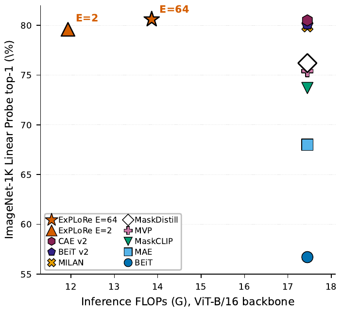
Every other published method sits bunched at 17.45 GFLOPs because they all ride vanilla ViT-Base/16, while ExPLoRe lands at the top-left of the plot, where the Soft-MoE structure gives a genuinely different inference profile and parameter count becomes a misleading proxy for cost. The reviewers were right, and the paper should have led with the compute framing from the start. That kind of feedback stings during the rebuttal window and leaves the paper better than the authors could have made it alone.

Scaling and downstream transfer#

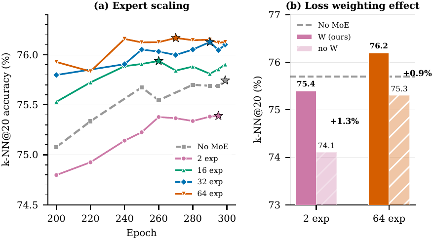
Panel (a) shows the scaling curve, with each line tracking a different expert count on k-NN between epochs 200 and 300. The shape is monotonic, with more experts giving higher final k-NN and the 64-expert model peaking at 76.2%. Panel (b) isolates the loss-coupling contribution at fixed expert count, where the weighted-versus-unweighted gap comes to +1.3% at 2 experts and +0.9% at 64, so the mechanism keeps paying for itself as the model grows.

Linear probe scales the same way, from 79.6% at 2 experts (+3.4% over the 76.2% baseline) to 80.6% at 64 (+4.4%). The linear-probe gap says more than the k-NN gap here, because k-NN measures frozen-feature distances while linear probe fits a classifier on the same frozen features, and a jump of 3 to 4 points on the latter means the routing reshapes the feature space toward better linear separability, a structurally different improvement from added capacity.

The Efficient Probing protocol (Psomas et al., ICLR 2026) gives even more direct evidence. EP is an attentive protocol that recovers patch-level information that CLS-aggregated probes under-measure, and under it the 2-expert model reaches 80.19% against 78.77% for the no-MoE baseline, a +1.41% gap and roughly three times the k-NN delta on the same backbones. One of the reviewers predicted exactly this pattern, with routing improving patch-level representations more than CLS-level ones, so CLS-aggregated metrics under-measure the gain. Fine-grained transfer on Food-101 shows the same behavior at +1.87%.

Dense prediction is where transfer gets harder. Semantic segmentation on ADE20K exposes the well-known MoE downstream problem, where routing patterns learned during pretraining can fight the uniform spatial coverage that dense prediction needs, and vanilla MoE finetuning lands 2.5 to 2.9 mIoU below the non-MoE baseline. Three adaptation recipes close the gap. Freeze Routing keeps the pretrained patch-expert assignments fixed during downstream finetuning, following ST-MoE, Expert Dropout applies dropout to expert outputs to prevent over-reliance on dominant experts, following Switch Transformer, and Freeze Attention freezes attention weights, also from ST-MoE. The full FR+FA+ExD stack recovers everything, reaching 52.8 mIoU on Token+Pixel and 51.1 on Token+CLS, each +0.3 over its non-MoE baseline. The recipes come from documented MoE-transfer work, and the same family closing the gap on both ImageNet finetuning and ADE20K segmentation suggests the difficulty lives in MoE transfer generally, with the underlying mechanism intact.

What I am less sure about#

A few caveats belong next to the headline numbers.

The three-loss extension, Token+CLS+Pixel, showed no measurable gain at default settings, with the MoE variant at 75.15% k-NN against 75.16% for the matched no-MoE three-loss baseline. The likely culprit is gradient-magnitude conflict between the three losses, which destabilizes specialization at the default entropy weight, and the asymmetric per-expert λ that worked for Token+Pixel did not transfer cleanly to three-loss training. This is one of the cleanest follow-up questions the paper leaves open.

The multi-seed coverage is thinner than ideal. Pretraining for 300 epochs on 4× H100 is expensive, and re-running 15 configurations at three seeds each was out of reach on our cluster budget. The mechanism-isolation deltas (+1.3% weighted versus unweighted, −1.6% for the detach) compare configurations that share pretraining randomness, so seed noise mostly cancels inside those comparisons. The headline +0.5% k-NN at 64 experts comes from a single run, though, since the seed study covers only the 2-expert model, and the compute-axis framing carries more of the argument than that small number does.

The 64-expert configuration deserves mixed feelings. The cost-quality story holds because of how Soft-MoE structures inference, yet 1.86 billion parameters trained from scratch for 300 epochs on ImageNet is hard to defend as practical for most uses. The 2-expert version is the practical recommendation, and the 64-expert one is mainly an existence proof that the mechanism keeps working at scale.

What I would do differently#

The mechanism-isolation comparisons should have existed from week three, and in practice they arrived around month eight. The detach ablation, the unweighted-MoE baseline, and the dispatch-versus-combine comparison each cost a fraction of a pretraining run, and having them early would have settled whether the dispatch-weight reuse was real, saved weeks of tuning entropy weights in the wrong λ region, and turned the combine-weight degeneracy from a multi-month detour into a two-day sanity check. The right diagnostic experiment ends the guessing, and without it a year can disappear into refreshing curves.

The FLOPs axis deserved the same treatment from day one. The cost-quality figure makes the story plainly a per-FLOP story, the parameter-axis framing undersells the method on the axis it actually competes on, and all three reviews raised it independently.

What is next#

ExPLoRe closes out the PhD work. I defended in April, joined an Amazon Robotics team in Berlin a few weeks ago, and the coming year will mostly involve language models for robotics, a different game from masked image modeling on ImageNet.

For anyone working on multi-objective pretraining who wants to try the dispatch-weight idea, the repo includes a smoke-test config that runs in about 15 minutes on a single GPU, and the paper has the full experimental detail. Issues are open, and the issue tracker gets faster answers than email.

The open question that interests me most is how the dispatch-weight idea generalizes outside MIM. Any multi-objective setup with spatial or token-level structure in its objectives is a candidate, with multi-task language modeling the most obvious and multi-modal pretraining close behind. Reports from anyone who tries are welcome in the comments below or on the repo.

How did this read?

👍Like0❤️Heart0🎉Celebrate0💡Insightful0

Comments

Loading comments...

0/1000Post comment